Exercise 1: The Equations of the Circle and the Sphere on Standard Form
In an ordinary $(O,\mathbf i, \mathbf j)$ coordinate system in the $(x,y)$ plane a circle can be described by the well-known quadratic equation:
$$\,(x-c_1)^2+(y-c_2)^2=r^2\,$$
where $(c_1,c_2)$ is its centre and $r$ its radius. We call this the standard form or standard equation.
A
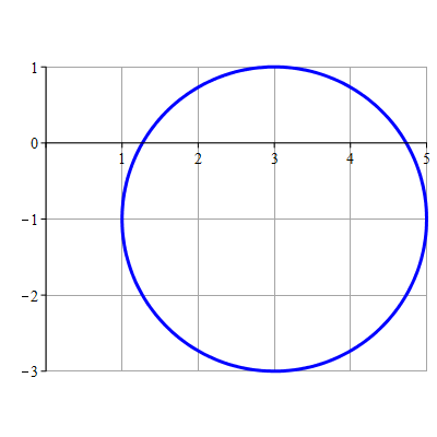
State the standard equation of the circle in the figure.
answer
$$\,(x-3)^2+(y+1)^2=4$$
B
A circle has the equation
$$\,x^2+y^2+8x-6y=0\,.$$
We cannot yet see that it actually is a circle. Bring it to standard form and state its centre and radius.
answer
Centre is $(-4,3)$. Radius is $5$.
C
A sphere in $(x,y,z)$ space has the equation
$$x^2+y^2+z^2-2x+4y-6z+13 = 0\,.$$
Bring it to the standard form
$$(x-c_1)^2+(y-c_2)^2+(z-c_3)^2=r^2,$$
and state its centre and radius.
answer
Centre is $(1,-2,3)$. Radius is $1$ (it is a unit sphere).
Exercise 2: The Standard Equations of the Three Typical Conic Sections
In the following questions we look at quadratic equations with more variables but without mixed terms. In these cases it is possible to proceed by “removing” the linear terms in the equations. This technique is called completing the square and was practiced in Exercise 1 with the simpler circles and spheres. The general goal with this topic is to become able to figure out and to characterize the shapes (conic sections) that the equations describe.
A
An general ellipsis in the $(x,y)$ plane centred at $(c_1,c_2),$ and with the semi axes $a$ and $b$ and the axes of symmetry $x=c_1$ and $y=c_2$ has the standard equation
Complete the square, bring the equation to standard form, and state the centre of the ellipse, the semi axes and the axes of symmetry.
hint
Plot the given equation using Maple’s implicitplot command to get an overview of what you are looking for.
hint
Consider the square theorem
$$(a+b)^2=a^2+b^2+2ab,$$
and “go backwards”.
hint
Look first at the square terms. E.g. $4x^2$. If this comes from a square of two terms, $(a+b)^2$ then it must be one of the squared parts, e.g. $a^2$. Which term squared gives $4x^2$? Then look at the “double product”, which can only be $8x$. Can we now determine which two terms $a$ and $b$ we have inside a squared bracket $(a+b)^2$?
hint
When you have rewritten to two terms in a squared bracket for both $x$ and $y$, then don’t forget to also “adjust” the constant. If in doubt, then do the math back to the original equation again to ensure that it fits.
answer
The ellipsis centre is $(-1,3).$
The semi axes are $a=1,\,b=2$.
The axes of symmetry are $x=-1,\,y=3.$
B
A general hyperbola in the $(x,y)$ plane centered at $(c_1,c_2),$ with the semi axes $a$ and $b$ and the axes of symmetry $x=c_1$ and $y=c_2$ has the standard equation
Complete the square, bring the equation to standard form, and state the centre of the hyperbola, the semi axes and the axes of symmetry.
answer
The hyperbola centre is $(2,-2).$
The semi axes are $a=2,\,b=2$.
The axes of symmetry are $x=2,\,y=-2.$
C
A general parabola in the $(x,y)$ plane with vertex $(c_1,c_2)$ and axis of symmetry $x=c_1$ has the standard equation
$$y-c_2=a(x-c_1)^2,$$
or alternatively, if it is not vertical but horizontal with the axis of symmetry $y=c_2$:
$$x-c_1=a(y-c_2)^2.$$
A specific parabola is given by the equation
$$\,2x^2+12x-y+17=0\,.$$
Complete the square, bring the equation to standard form, and state the vertex of the parabola and the axis of symmetry.
answer
The vertex is $(-3,-1).$
The axis of symmetry is $x=-3.$
Exercise 3: Identification of a Conic Section
In an ordinary $(O,\mathbf i, \mathbf j)$ coordinate system in the $(x,y)$ plane a conic section is given by the following quadratic equation with two variables:
$$9x^2+16y^2-24xy-40x-30y+250=0.$$
We cannot readily see from the equation which shape (which conic section) is represents (if any). In the following questions we will determine its type and characterize it as in the previous exercise.
A
The left-hand side of the quadratic equation can be split into three components:
A quadratic form. Let’s denote it $k(x,y)$.
Linear terms forming a linear polynomial.
A constant.
State the quadratic form and determine its Hessian matrix.
In a new coordinate system $(O,\mathbf q_1,\mathbf q_2),$ that appears by rotating$(O,\mathbf i, \mathbf j),$ the equation for the given conic section is changed so as to be without mixed terms. State the orthonormal basis that defines this new rotated coordinate system, and determine the new equation for the conic section.
hint
Use the columns of $\mQ$ as the new basis.
We have already changed the quadratic form to the new $(x_1,y_1)$ coordinates. We are only missing the linear terms $-40x-30y\,.$
hint
We have the change-of-basis relation $\displaystyle{\begin{matr}{r}x\newline y\end{matr}=\mathbf Q\,\begin{matr}{r}x_1\newline y_1\end{matr}}.$ From this we see how $x$ and $y$, respectively, can be expressed by $x_1$ and $y_1$ which can be inserted into $-40x-30y\,.$
hint
When you have finished both the quadratic and the linear terms, then don’t forget the constant.
The given conic section has in the new coordinate system the equation
$$25x_1^{\,2}-50y_1+250=0\,.$$
E
Which type of conic section are we talking about? Characterize it, both in terms of the new and in the original coordinate system. Illustrate with Maple.
hint
You must now use the techniques such as completing the square from the previous exercises.
hint
When rewritten, compare the standard form of the equation with those defined in the previous exercise.
answer
The equation of the conic section can immediately be rewritten to
$$y_1-5=\frac 12\,x_1^{\,2}.$$
This is a parabola with the vertex $(x_1,y_1)=(0,5)$ and the $\,y_1$ axis as its axis of symmetry.
In the given (the original) coordinate system the vertex is found at $\displaystyle {\begin{matr}{r}x\newline y\end{matr}=\mathbf Q\,\begin{matr}{r}0\newline 5\end{matr}=\begin{matr}{r}4\newline 3\end{matr}}.$
A direction vector of the axis of symmetry in the new coordinate system is $\mathbf e=(0,1).$ In the original coordinates, this vector is $\displaystyle{ \mathbf Q\,\begin{matr}{r}0\newline 1\end{matr}=\begin{matr}{r}\frac 45\newline \frac 35\end{matr}}.$ Thus the axis of symmetry has the parametric representation
In an ordinary orthogonal $(x,y)$ coordinate system a curve is given by the equation:
$$52x^2+73y^2-72xy-200x-150y+525=0.$$
Describe the type and position of the curve, and provide parametric representations for any axes of symmetry.
hint
State the quadratic form on matrix form $\,\begin {matr}{cc} x & y \end{matr}\mA\begin{matr}{rr} x \newline y \end{matr}\,$ and diagonalize $\,\mA\,.$
hint
State the equation that the conic section has in a new $(x_1,y_1)$ coordinate system consisting of the origin and the new orthonomal basis. First we deal with the quadratic form, then the linear terms, and then finally will add the constant.
hint
The conic section has in the new $(x_1,y_1)$ coordinate system the equation
$$100x_1^{\,2}+25y_1^{\,2}-250y_1+525=0\,.$$
Now complete the square and you should be able to identify the type of this conic section and should be able to read from it all the relevant characteristic to mention.
answer
In the new coordinate system the conic section has the equation
$$\frac {x_1^{\,2}}1+\frac{(y_1-5)^2}{4}-1=0$$
or similar (depending on your choice of a new basis). So, it is an ellipsis with semi axes $a=1$ and $b=2$ and centre at $(0,5).$
In the given coordinate system the centre is $(4,3),$ and the axes of symmetry are described by the following parametric representations:
$$\text{Major axis:}\qquad (x,y)=(4,3)+t_1\big(\frac 45,\frac 35\big)\quad\text{ where } \quad t_1\in\reel$$
Plot using Maple the conic section, both in the new and the original coordinate system, as well as the axes of symmetry. Compare with a plot of level curves for the polynomial
$$f(x,y)=52x^2+73y^2-72xy-200x-150y+525\,.$$
In particular, consider the level curve corresponding to a height of $0$!