Find the eigenvalues and the corresponding eigenspaces of the system matrix, and - using this - state the general real solution to the system.
Find the solution to the system that satisfies $\,x_1(0)=0\,$ and $\,x_2(0)=3\,.$
answer
The eigenspaces are $E_3=\mathrm{span}{(4,1)}\,$ and $E_{-3}=\mathrm{span}{(-2,1)}\,.$ All multiplicities are $1$.
Thus the general real solution can be written as:
We are given the following system of differential equations:
\begin{equation}
\begin{matr}{rr} x_1’(t) \newline x_2’(t) \end{matr} =
\begin{matr}{rr} 2 & -5\newline
1 & -2 \end{matr}
\begin{matr}{rr} x_1(t) \newline x_2(t) \end{matr}, \quad t \in \reel
\end{equation}
Find the eigenvalues and the corresponding eigenspaces of the system matrix, and - using this - state the general complex solution to the system.
Now state the general real solution to the system.
Now we will find the solution to the system that satisfies $\,x_1(0)=0\,$ and $\,x_2(0)=3\,.$ Consider the following: Do we get the same solution if we find the solution using the general complex solution as we get using the general real solution?
answer
The eigenspaces are $E_i=\mathrm{span}{(2+i,1)}\,$ and $E_{-i}=\mathrm{span}{(2-i,1)}\,.$ All multiplicities are $1$.
The general real solution:
$$ \begin{matr}{rr} x_1(t) \newline x_2(t) \end{matr} = c_1 \begin{matr}{rr} 2\cos t-\sin t \newline \cos t \end{matr} + c_2 \begin{matr}{rr} \cos t + 2\sin t \newline \sin t \end{matr} , \quad (c_1,c_2) \in \reel^2$$
Given the system of differential equations
\begin{equation}
\begin{matr}{rr} x_1’(t) \newline x_2’(t) \end{matr} =
\begin{matr}{rr} 2 & 1\newline
-4 & -2 \end{matr}
\begin{matr}{rr} x_1(t) \newline x_2(t) \end{matr}, \quad t \in \reel
\end{equation}
Find the eigenvalues and the corresponding eigenspaces of the system matrix, and - using this - state the general real solution to the system.
Find the solution to the system that satisfies $\,x_1(0)=0\,$ and $\,x_2(0)=3\,.$
answer
There is only one eigenspace $E_0=\mathrm{span}{(-\frac{1}{2},1)}\,.$ The multiplicities are: $\mathrm{am}(0)=2$ and $\mathrm{gm}(0)=1$. The system matrix cannot be diagonalized by similarity transformation.
The general real solutions is:
Exercise 2: Homogeneous Linear System of Differential Equations
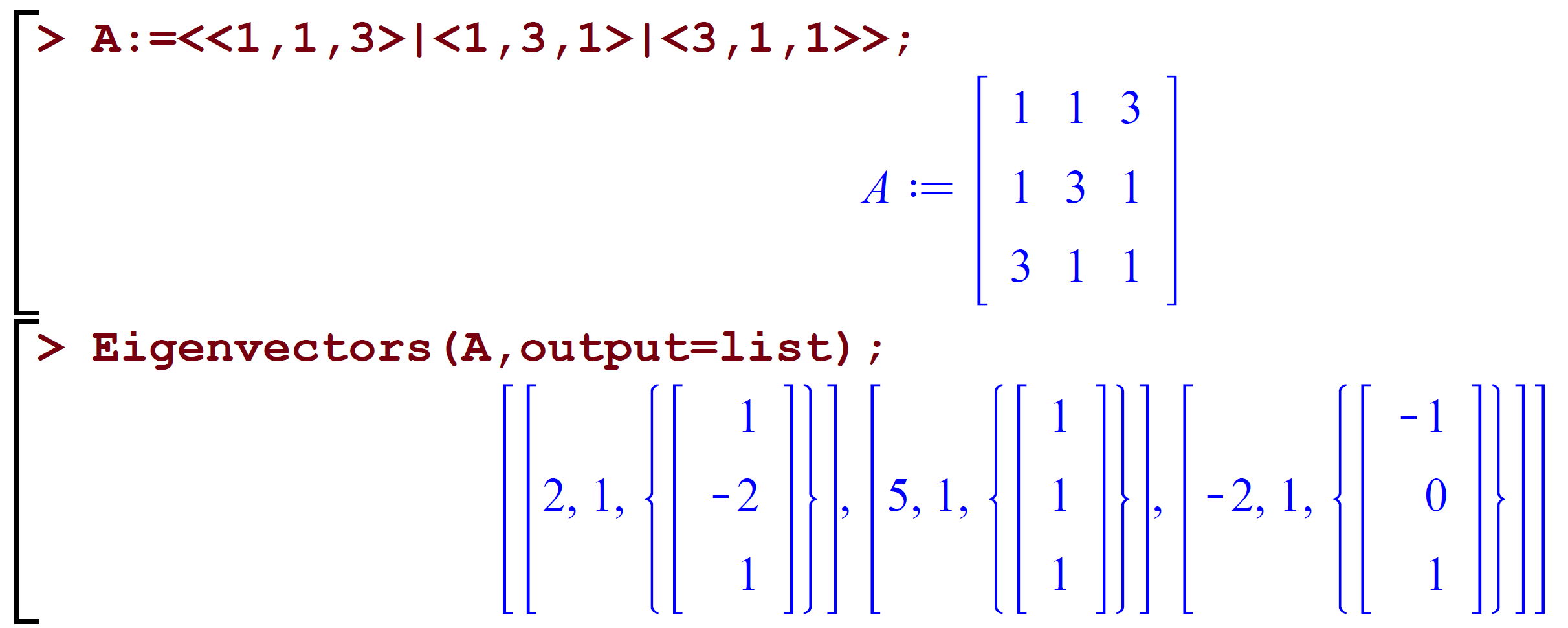
A homogeneous linear system of differential equations consisting of three equations with the unknown functions $\,x_1(t),x_2(t)\,$ and $\,x_3(t)\,$ (with $t\in\reel$) has the system matrix $\mA$ that has been treated in Maple like this:
A
How do the three differential equations look on their ordinary form (not the matrix-form).
B
State the general real solution both on matrix form and on ordinary form.
Exercise 3: The Structural Theorem. Theory
Let $\,C^{\infty}(\Bbb R,\Bbb C)\,$ denote the functional vector space of infinitely-many-times differentiable complex functions of a real variable with $\,\Bbb C\,$ as the corresponding scalar field. For $\,t\in \reel\,$ the functions $\,\cos(t),\,\e^{2it}\,$ and $\,t^3\,$ are examples of vectors in the vector space.
Denote the vector space of pairs of such functions by $\,C^{\infty}(\Bbb R, \Bbb C))^2= \lbrace(x,y) ~|~ x \in C^{\infty}(\Bbb R,\Bbb C), y \in C^{\infty}(\Bbb R,\Bbb C) \rbrace$.
Now we consider the map $\,f:(C^{\infty}(\Bbb R, \Bbb C))^2\rightarrow (C^{\infty}(\Bbb R,\Bbb C))^2\,$ given by
where $\,\mA\,$ is a real $2\times2$ matrix, $\,\mx(t)=(x_1(t),x_2(t))\,$ and $\,\mx’(t)=(x_1’(t),x_2’(t))\,.$
A
Show that $\,f\,$ is linear.
hint
$f\,$ must satisfy the two linearity requirements:
$f(\mx(t)+\my(t))=f(\mx(t))+f(\my(t))\,.$
$f(k\mx(t))=kf(\mx(t))\,.$
B
Explain that systems of differential equations like the ones that are treated in Exercise 1 above, can be considered to be homogeneous vector equations of the type
$$\,f(\mx(t))=\mnul\,.$$
C
How can the structural theorem be applied to vector equations of the type
$$\,f(\mx(t))=\mathbf q(t)\,$$
where $\,\mathbf q(t)\in (C^{\infty}(\Bbb R,\Bbb C))^2\,.$ Give a precise formulation.
Exercise 4: The Structural Theorem. By Hand
A
Find the general solution to the system of differential equations
\begin{equation}
\begin{matr}{rr} x_1’(t) \newline x_2’(t) \end{matr} = \begin{matr}{rr} 1 & 1\newline 0 & -2 \end{matr}\cdot \begin{matr}{rr} x_1(t) \newline x_2(t) \end{matr}\,\,,\quad t\in \reel\,.
\end{equation}
hint
Apply the solution formula in Theorem 17.2 in eNote 17.
and then state the general real solution to the system.
hint
Concerning the guess: First find $\,x_2(t)\,$ by guessing a first-degree polynomial $\,at+b\,$ based on the last equation. Substitute the result into the first equation, and now find $\,x_1(t)\,$ by again guessing a first-degree polynomial.
hint
Concerning the general solution: Use the structural theorem.
Write the system on matrix form. Find the eigenvectors and the corresponding eigenvalues of the system matrix.
B
Find using Maple’s dsolve the general solution to the system of differential equations. How can the solution be interpreted, on the one hand in the context of eigenvectors and eigenvalues of the system matrix and on the other hand in the context of the structural theorem?
C
Plot the solution that satisfies $\,x_1(0)=10\,$ and $\,x_2(0)=5\,,$ first for $\,t\in \left[\,0,10\,\right]\,$ and then for $\,t\in \left[\,10,20\,\right]\,$ and comment on the result.
Exercise 6: Modelling of a Physical Situation
In this exercise you yourself will model from scratch a physical situation using Maple and make experiments with the model. This, together with Exercise 5, is a warm-up to Theme Exercise 4. Here we consider a homogeneous system, whereas the Theme Exercise concerns inhomogeneous systems.
The procedure is that you read the text and execute the commands in the Maple sheet one at a time - do not use the execution button !!! in Maple that will execute the entire sheet at once. When you have answered a question then you are welcome to open the Solution tab to see the suggested solution.
A
Download the file eMaple2 and have fun with the modelling.
Exercise 7: Existence and Uniqueness. Advanced.
Again we consider the following system of differential equations from Exercise 1:
Explain that for every 3-tuple of numbers $(t_0,a_0,b_0)$ exactly one solution $(x_1(t),x_2(t))$ to the system exists such that $x_1(t_0)=a_0$ and $x_2(t_0)=b_0$.
hint
Is it possible to find two different solutions that satisfy $\,x_1(t_0)=a_0\,$ and $\,x_2(t_0)=b_0\,$?
hint
Insert $\,x_1(t_0)=a_0\,$ and $\,x_2(t_0)=b_0\,$ into the general solution found for the system. How many different values can $\,c_1\,$ and $\,c_2\,$ have?
hint
$\,c_1\,$ and $\,c_2\,$ are unique. Why?
hint
Consider the general solution found as a system of equations where $\,c_1\,$ and $\,c_2\,$ are unknowns. Show that only one solution exists (the coefficient matrix is regular).
$c_1$ and $c_2$ are uniquely determined and depend on the 3-tuple $(t_0, a_0, b_0)$.
B
Given an arbitrary 3-tuple $\,(t_0,a_0,b_0)\,$. Consider if there always - for systems of differential equations of the type considered in the exercise above - exists exactly one solution $\,(x_1(t),x_2(t))\,$ to the system such that $x_1(t_0)=a_0$ and $x_2(t_0)=b_0$.